By Humtech RITCs on February 10, 2025
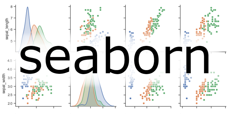
There are a few Python libraries that enable researchers to create exceptional visualizations. Among these, I’d like to introduce Seaborn—a versatile and user-friendly library specifically designed for crafting informative and visually appealing statistical plots. Built on top of Matplotlib, Seaborn streamlines the creation of advanced data visualizations and elevates the aesthetic quality of standard graphs. Its integration with pandas makes it an ideal choice for data analysis and exploratory data visualization. According to Seaborn’s official introduction: “Seaborn’s plotting functions operate on data frames and arrays containing entire datasets, internally performing the necessary semantic mapping and statistical aggregation to produce informative plots. Its dataset-oriented, declarative API allows users to focus on the meaning of the different elements in your plots, rather than on the details of how to draw them.“
Below, I will present four examples of what Seaborn can do.
- #Let’s get the test data ready
- import pandas as pd
- input_data = pd.read_csv(“Recoded_CSS_data.csv”)
- data = input_data[“collgpa_standardized”].round(2)
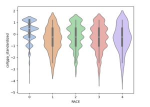
Violin Plot
A violin plot is a powerful data visualization tool that combines the features of a box plot and a kernel density plot. It provides a comprehensive view of the distribution of a dataset by displaying both the summary statistics (e.g., median, quartiles) and the probability density of the data at different values. Compared to a box plot, a violin plot reveals the full distribution shape, making it particularly useful for comparing multiple groups or datasets. It is commonly used in exploratory data analysis to detect patterns, differences, or anomalies in the data.
Here’s an example of generating a violin plot with Seaborn:
- import seaborn as sns
- import matplotlib.pyplot as plt
- #generate the violin plot
- sns.violinplot(x=input_data[“RACE”],y = input_data[“collgpa_standardized”].round(2),palette=’pastel’)
- plt.show()
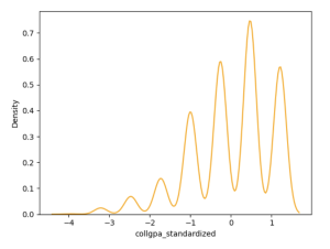
KDE Plot
A Kernel Density Estimation (KDE) Plot is a statistical tool used to estimate the probability density function of a continuous random variable. It provides a smoothed representation of the data’s ›distribution, making it easier to visualize underlying patterns and trends compared to a histogram. KDE plots work by placing a kernel (a smooth, symmetric function, typically Gaussian) over each data point and summing these kernels to create a continuous density curve. It is particularly useful for analyzing the shape of data distributions.
Here’s an example of generating a KDE plot with Seaborn:
- import seaborn as sns
- import matplotlib.pyplot as plt
- sns.kdeplot(input_data[“collgpa_standardized”].round(2),color = “orange”)
- plt.show()
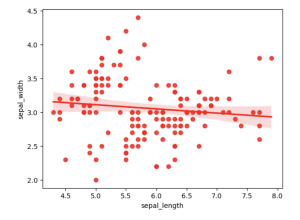
Scatter Plot
A Scatter Plot is a type of data visualization used to demonstrate the relationship between two variables. Each point in the plot represents an observation, with its position determined by the values of the two variables: one on the x-axis and the other on the y-axis. Scatter plots are widely used to identify correlations, patterns, clusters, or outliers in data, and they can also incorporate observations from higher dimensions using additional attributes like color, size, or shape.
Here’s an example of generating a Scatter plot with Seaborn:
- import seaborn as sns
- import pandas as pd
- import matplotlib.pyplot as plt
- #loading the example data
- df = sns.load_dataset(‘iris’,data_home = ‘seaborn-data’,cache=False)
- sns.regplot(x= df[“sepal_length”], y = df[“sepal_width”],color = “red”)
- plt.show()
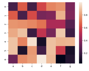
Heat Plot
A Heat Plot, or a Heatmap, is a data visualization technique that uses color to represent values in a matrix or muti-dimensional data set. Each cell in the heatmap corresponds to a value, and the intensity or hue of the color indicates the magnitude of that value. Heatmaps are particularly useful for identifying patterns, correlations, or anomalies in data, making them popular for visualizing relationships in tables, time series data, or correlations between variables.
Here’s an example of generating a heatmap with Seaborn:
- import numpy as np
- import pandas as pd
- import seaborn as sns
- #loading the example data
- df = pd.DataFrame(np.random.random((7,7)),columns = [“a”,”b”,”c”,”d”,”e”,”f”,”g”])
- #generate the default heatmap
- p1 = sns.heatmap(df)
About the Author:
Tianji Jiang (he/him) is currently pursuing a Ph.D. in Information Studies at the University of California Los Angeles (UCLA)’s School of Education and Information Studies program. His passion pivots around advocating for the openness and sharing of research data, with a specific focus on how libraries can contribute to the research data life cycle and maximize the benefits of open data. He has worked as a RITC (Research and Instructional Technology Consultant) since 2022.
Banner image source; all other images by author